Self-similarity

When I think of self-similarity, the first thing that comes to my mind is Romanesco broccoli. The shape is indeed self-similar and mathematically closely related to a spiral. In simple words, self-similar means that no matter how much you zoom in, you will see the same shape. This thinking can then be applied not only to shapes (sets, functions), but also to equations. Let’s see how!

Self-similarity of functions

Formally, a function $f(x)$ or a set $S$ is self-similar if scaling the input by a factor $\lambda$ changes the output in a predictable, proportional way:

$f(\lambda x) = \lambda^k f(x),$

where $k$ is a scaling exponent. Here are some intuitive real-world examples, some of which I am sure all of us have seen somewhere.

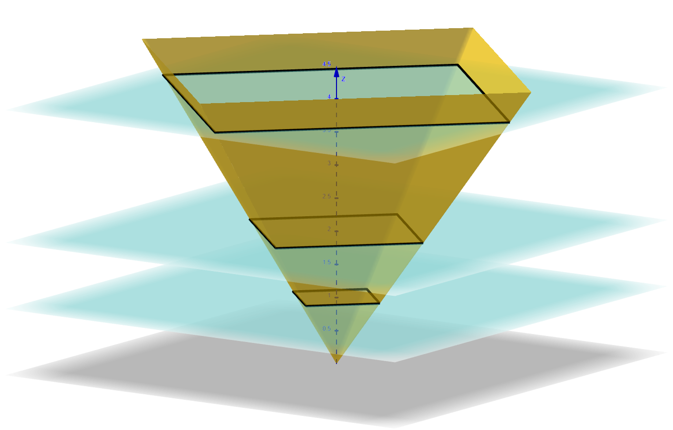
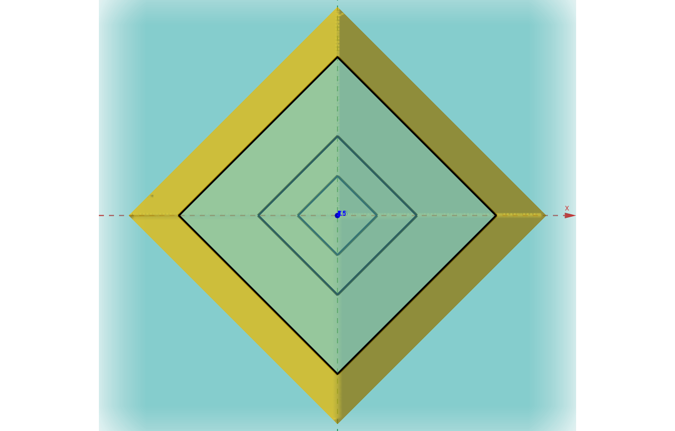
This is a standard definition of a homogeneous function of degree $k$ that we learn in Calculus. A simple example of a self-similar shape is that of a pyramid given by the function

\(f(x,y)=|x|+|y|\) .

The function is homogeneous of degree 1, with horizontal cross-sections given by the level sets

\(L_c = \{ (x,y): |x|+|y|=c \}\) ,

which are diamonds (squares rotated by 45°). Now, looking down the $z$-axis, if we zoom in by a factor of 2, then we will be looking at the level curves of

\((1/2) f(x, y) = (1/2) c = (1/2) (|x|+|y|) = |x/2|+|y/2| = f(x/2, y/2)\) ,

which implies that

\(L_{c/2} = (1/2) L_c\) .

The level curves, diamonds, are exactly the shape, scaled by a factor of 1/2.

This means that if you view the pyramid from above (along the $z$-axis) and zoom in by a factor of 2, you will see the same diamond shape with half the side length. Moreover, this remains true for any zooming factor: no matter how much you zoom in or out, the level sets keep the same shape, differing only by scale, i.e.,

\(L_{\lambda c} = \lambda L_c\) .

Thus, the top view of the pyramid is self-similar, just like in the figure.

Self-similarity of curves

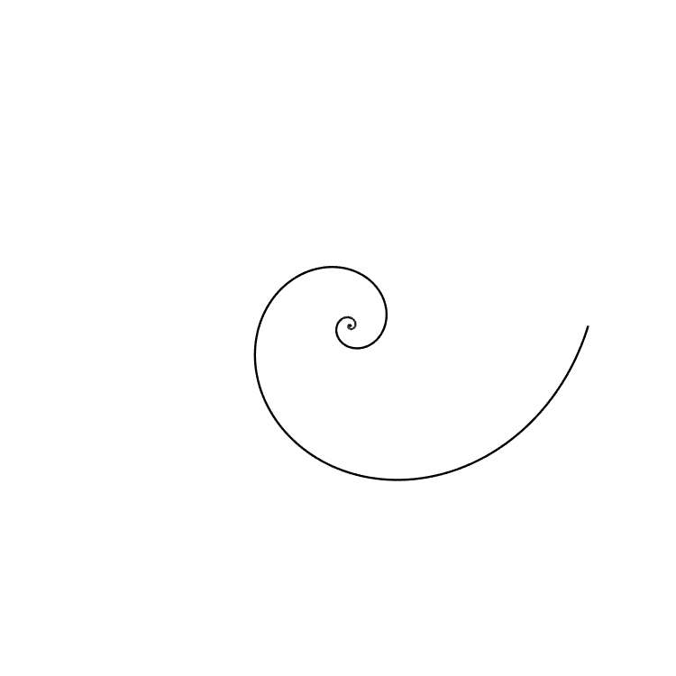
Another interesting and closed-form example is the logarithmic spiral, which has exact geometric self-similarity. In the polar form, it can be expressed as

\(r(\theta)=r_0 e^{b\theta}\) ,

where $r_0>0$ is the initial radius, $b\ne0$ controls how tightly the spiral winds and $\theta$ is the polar angle.

So if we scale or zoom the spiral by a factor $\lambda$, i.e.,

\(r\rightarrow \lambda r\) ,

then

\(\lambda r(\theta) = r_0 e^{b (\theta+\Delta \theta)} = r(\theta+\Delta \theta)\) , where $\Delta \theta = \frac{\ln \lambda}{b}$.

It turns out that when $\Delta \theta = \frac{\pi}{2}$, and $\lambda = \frac{1+\sqrt{5}}{2}$, the Golden ratio, then the corresponding spiral is called the Golden spiral. Voilà! That’s the shape of a Romanesco broccoli!

This means zooming the entire curve is equivalent to rotating it; the shape remains the same, but not the size.

Left: Messier 74. Image credit: www.nasa.gov. Right: Golden spiral.

Self-similarity of equations

After seeing self-similarity in both functions and curves, it’s natural to wonder whether these patterns appear as solutions of differential equations. In fact, the answer is yes, and in the case of a logarithmic spiral, it’s a simple Ordinary Differential Equation (ODE),

\(r^\prime = \frac{dr}{d\theta}=b r(\theta)\) .

This equation can be derived by imposing that as we move along the curve $r(\theta)$, the tangent vector always makes a constant angle with the radial direction (the line from the origin to the point).

More generally, for Partial Differential Equations (PDEs), imposing a self-similar form often transforms the PDE into an ODE. For example, the heat equation

\(u_t = u_{xx}\) ,

is invariant under the scaling

\(x \rightarrow \lambda x, \quad t \rightarrow \lambda^2 t\) ;

that is, if $u(x,t)$ solves the equation, then so does (under constant energy assumption)

\(u_\lambda(x, t) = \lambda u(\lambda x, \lambda^2 t)\) .

In this case, a natural self-similar form is given by

\(u(x,t) = t^{-1/2} u\left(\frac{x}{\sqrt{t}}, 1 \right) = t^{-1/2} F\left(\frac{x}{\sqrt{t}}\right) = t^{-1/2} F(\xi)\) ,

where the profile $F$ satisfies

\(F^{\prime\prime} + \frac{\xi}{2} F^\prime + \frac12 F=0\) , solving which gives

\(F(\xi) = C e^{-\xi^2/4} \implies u(x,t) = \frac{C}{\sqrt{t}} e^{-x^2/4t}\) ,

the fundamental solution of the heat equation.

Let’s now consider a PDE whose solution is not a scalar but an evolving arc-length parameterised curve, $\gamma$ satisfying

\(\gamma_t = \kappa \mathbf{n}\) ,

where $\kappa$, is the curvature and $\mathbf{n}$, the normal vector. This equation is known as Curve shortening flow (CSF) and explains the evolution of a curve whose velocity vector has the tangential component equal to zero.

Although using the two-dimensional Frenet frame, one can write $\gamma_t=\gamma_{ss}$, this is not the heat equation, as the arc-length coordinate $s$ changes with time. However, just as with the heat equation, it is natural to ask whether the flow admits self-similar solutions.

It turns out that CSF is invariant under rotations and scalings, so we look for solutions of the form

\(\gamma(s, t) = \lambda(t) R_{\omega(t)} \Gamma(s)\) ,

where $\lambda(t)$ controls the scaling, $R_{\omega(t)}$ is a rotation by angle $\omega(t)$, and $\Gamma(s)$ is the fixed shape we want to determine.

Substituting the above ansatz in the CSF gives the ODE for $\Gamma$:

\(\Gamma^{\prime\prime} = p \Gamma + q J \Gamma\) ,

where $J\Gamma$ is a 90º rotation of $\Gamma$ and $p$, $q$ are constants depending on the rate of scaling and rotation.

By writing $\Gamma(s) = (x(s), y(s))$ and $z=x+iy$, the above ODE becomes

\(z^{\prime\prime} = (p+iq) z\) ,

whose solution in the polar form is

\(r(\theta) = r_0 e^{b\theta}, \quad \text{where} \quad b = Re{(u)}/Im{(u)}, \quad \text{and} \quad u = \sqrt{p+iq}\) .

That is, the logarithmic spiral, or our very…

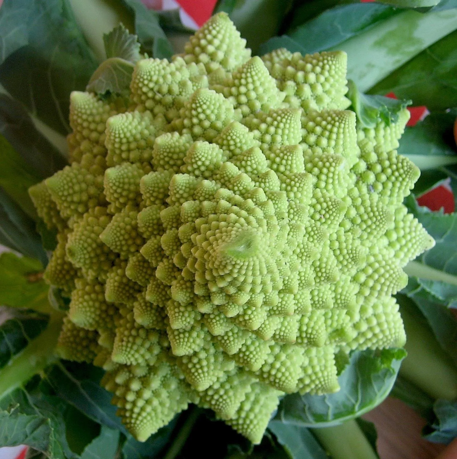
Image credits: wonderhowto.com